Model optimization methods to cut latency, adapt to new data

Lightweight model implementation: Overview

• How can prediction latency be kept to a minimum in a real-time data processing system while guaranteeing acceptable accuracy?
• A complex model with high accuracy generally incurs high prediction latency when deployed in real-time systems, leading to degraded system performance with the further consequences of potential business loss.
• A lightweight model with acceptable accuracy is trained and deployed to make real-time predictions.
• Application. A statistical or a simple machine learning algorithm, such as naive Bayes, is used to train a predictive model that is then deployed in the real-time system to make low latency predictions.

Lightweight model implementation: Explained

Problem

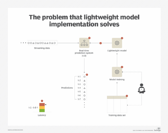
A real-time data processing system, such as an event stream processing (ESP) system, requires minimum possible delay from the time the data gets ingested to the time the predictions become available. However, with the aim of achieving maximum possible accuracy, which generally results in a complex model, prediction time increases. Although the system generates accurate results, by the time the results are accessible the window of opportunity may already have closed. In a very high-velocity data processing system, such as with an IoT-driven system, not only does this incur prediction lag but also results in excessive use of memory and processing resources. (See Figure 1.)

Solution

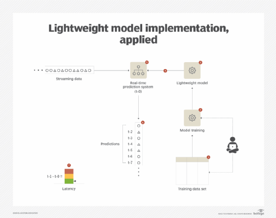
A real-time system suffers from the limitations described by the speed consistency volume (SCV) principle. To be able to operate at high velocity (S) while making sure that all data gets processed (V), the accuracy of the predictions needs to be relaxed (C) by employing a lightweight model. Such models are either probability-based or use a linear classifier to keep the memory and computation overhead to a minimum. Although the accuracy of such models is not on par with complex models, their ability to predict faster offsets the reduced accuracy. To reduce false positives or to gain further insight into the data points, the data points can then be fed to a more complex model operating at near-real-time that may make use of other contextual data not available to the real-time prediction pipeline.

Application

Based on whether the nature of a problem is regression or classification, a lightweight algorithm is chosen. With regression, linear regression or a pruned decision tree can be used; with classification, logistic regression, linear support vector machine (SVM) or naive Bayes can be used to train a model in an offline manner by making use of as much data as possible. The trained model can then be deployed in the real-time system.

With IoT devices, once the lightweight classification model predicts that a data value falls within a class of interest or if the regression model's prediction falls within the range of interest, one strategy to gain insight or to confirm the model's prediction is to reconfigure the IoT device to gather more granular data that can then be fed to complex models, such as kernel SVM. The same strategy can also be employed for non-IoT systems.

The use of complex models as a second stage may also be required when there is a requirement for the prediction to be explainable to a decision maker or a third-party, such as the detection of fraudulent bank transactions. Models based on rule-centered algorithms, such as decision trees and classification rules, can be used in such scenarios. 

The lightweight model implementation pattern can further benefit from the application of the incremental model learning pattern as it helps keep retraining time and resources to a minimum, which further helps when updating the productionalized model more frequently, thereby achieving more accurate predictions. (See Figure 2.)

Incremental model learning: Overview

• How can a model be retrained without having to be trained from scratch when new data is acquired?
• After the initial training of a model, it is imperative that the model is retrained as new data becomes available. However, this retraining can take a long time and can use excessive processing resources, thereby risking the availability of an up-to-date model in a timely fashion.
• A classifier that is not dependent on historical data and only requires new data for retraining is deployed to make predictions.
• An incremental classifier such as naive Bayes is used where the model is updated based on new example data only without the need for regenerating the whole model from scratch.

Incremental model learning: Explained

Problem

After the initial training and deployment of a model, the effectiveness of the model remains within the expected bounds as long as the model's input remains comparatively similar in its behavior when compared with the data that was originally used to train the model.

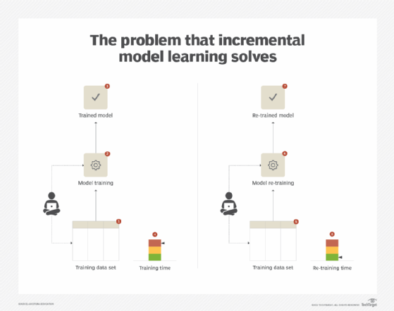
However, the characteristics of the input data often change over time. Consequently, as prescribed by the frequent model retraining pattern, the model needs to be retrained. Based on the available processing resources and the required retraining frequency, the retraining can take considerable time and use a large volume of processing resources. This increases the potential of using a less-accurate model for longer in the production system before the up-to-date model becomes available. (See Figure 3.)

Solution

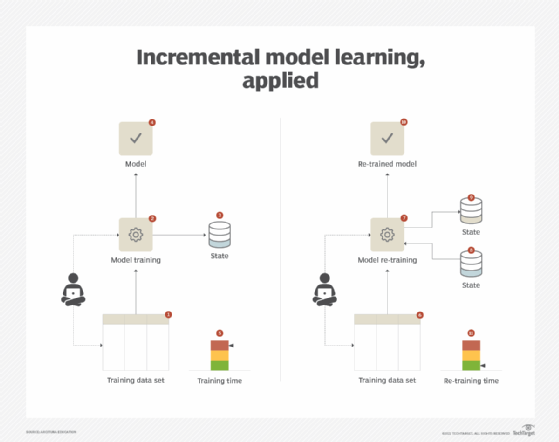
The increased use of processing resources, which translates into both increased cost and time, can generally be attributed to the re-computational nature of the underlying algorithm used for model training. Such an algorithm requires the complete data set for retraining purposes. For example, with K-nearest neighbors (K-NN), whenever a new data point is fed to the model, the algorithm scans the entire data set to find the K number of the most similar data points based on the Euclidean, Hamming or Cosine distance measures. In order to decrease the retraining time, an incremental classifier is employed. Such a classifier is built on top of an algorithm that does not need to go through the entire data set again whenever the model needs to be retrained. Instead, the model keeps the previous state and updates the state based on computations made on the new data.

Application

An incremental machine learning algorithm such as naive Bayes is used to train a model based on the entire data set at the beginning. However, after the initial deployment of the model, once there is a need to retrain the model, only the newly acquired data is fed into the model retraining process. The underlying algorithms are able to support this functionality as they generally make some assumptions and are probabilistic rather than deterministic.

For example, naive Bayes assumes that all features are equal in importance and calculates the probability of each feature independently of other features. This way, it does not need to recalculate the probabilities from scratch and can keep the state of previously computed probabilities and only needs to update the probabilities when new examples are fed.

The application of this pattern is dependent upon the availability of the incremental version of the underlying algorithm, which may not be possible in all scenarios. Also, business requirements may impose constraints that make the use of incremental algorithms unsuitable. For example, replacing a decision-tree classification model with a naive Bayes classification model may not be a possibility if the business requires the use of an explainable model rather than a black box model (Figure 4).

This concludes our 13-part series on how machine learning works. This subset of AI is now in use throughout IT and integral to the smooth operation of many popular applications. Whether you're looking to break into the ML job market, or just curious about how ML makes our world go round now, we hope this series has proved enlightening and provided a solid grounding in this essential tool. If you're interested in developing your expertise further, please check out this training to become a certified machine learning specialist.